


General relativity
Dr. Gyula Bene
Department for Theoretical Physics, Loránd Eötvös University
Pázmány Péter sétány 1/A, 1117 Budapest
1. week
Introduction
Literature
Original articles:
- A.Einstein, Die Feldgleichungen der Gravitation, Berl.
Ber. 44 (1915) 844.
Eötvös Loránd szerepe: az Eötvös-kísérlet, 1908-1909.
- R. v. Eötvös, Mathematishe und Naturwissenschaftliche
Berichte aus Ungarn, 8,65,1890.
- R. v. Eötvös, Verhandlungen der 16. Allgemeinen Konferenz
der Internationalen Erdmessung (London-Cambridge, 21-29 September 1909)
- R. v. Eötvös, D. Pekár, E. Fekete: Beiträge zum Gesetz
der Proportionalität von Trägheit und Gravität; a Beneke Alapítványhoz
benyújtott pályamű, 1909.
Preliminaries: special relativity (A.Einstein,
1905)
Events, reference frame, inertial frame
Lorentz transform
\[\begin{align}x'=\frac{x-vt}{\sqrt{1-\frac{v^2}{c^2}}}\end{align}\]
\[\begin{align}y'=y\end{align}\]
\[\begin{align}z'=z\end{align}\]
\[\begin{align}t'=\frac{t-\frac{v}{c^2}x}{\sqrt{1-\frac{v^2}{c^2}}}\end{align}\]
Maxwell's equations are covariant to Lorentz transforms
\(\bf{\rightarrow}\)
The velocity of light is independent of the chosen inertial frame. Michelson,
1881, Michelson and Morley, 1887.
There is no distinguished inertial frame (principle of relativity)
\(\bf{\rightarrow}\)
Lorentz transform expresses a basic symmetry of spacetime.
Interval:
\[\begin{align}s^2=c^2t'^2-{\bf{r'}}^2=c^2t^2-{\bf{r}}^2\end{align}\]
Otherwise:
\[\begin{align}
s^2=g_{ik}x^ix^k
\end{align}\]
where
\[\begin{align}
x^0=ct,\;x^1=x,\;x^2=y,\;x^3=z
\end{align}\]
and
\[\begin{align}
g_{ik}={\rm diag}(1,-1,-1,-1)
\end{align}\]
Proper time:
\[\begin{align}\tau^2=t^2-\bf{r}^2/c^2\end{align}\]
Minkowski space. Timelike, spacelike, lightlike intervals.
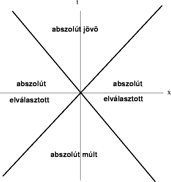
|
Fig. 1. Causal structure of Minkowski space:
light cones separate timelike and spacelike regions.
Time is not absolute: the relativity of simultaneity
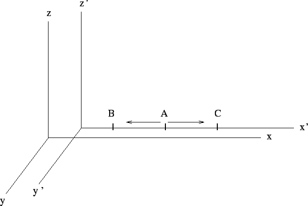
|
Fig. 2. Simultaneity is relative: light signals
arrive at B and C in coordinate frame K' at the same time while in frame K at
different times.
\[\begin{align}
x_1'\ne x_2',\; t_1'=t_2' {\;\bf\rightarrow\;} t_1\ne t_2
\end{align}\]
because Lorentz's transform implies
\[\begin{align}
t_2-t_1=\frac{\frac{v}{c^2}(x_2'-x_1')}{\sqrt{1-\frac{v^2}{c^2}}}
\end{align}\]
Lorentz contraction:
The two ends of a moving meter-stick measured in frame K: \( (0,0) \)
and \( (0,L) \) (notation meaning \( (t,x) \) )
In comoving frame K' the same events are \( (0,0) \)
and \( (t',L_0) \).
Applying Lorentz's transform we have
\[\begin{align}
L_0=\frac{L}{\sqrt{1-\frac{v^2}{c^2}}}\;,
\end{align}\]
i.e.
\[\begin{align}
L=L_0\sqrt{1-\frac{v^2}{c^2}}\;.
\end{align}\]
Time dilatation:
Given pointer states of a moving clock (0 and \(\tau\) )
measured in frame K : \( (0,0) \)
and \( (t,x) \)
In comoving frame K' the same events are \( (0,0) \)
and \( (\tau,0) \)
According to Lorentz's transform
\[\begin{align}
t=\frac{\tau}{\sqrt{1-\frac{v^2}{c^2}}}
\end{align}\]
Twin paradox
Transformation of velocities:
\[\begin{align}
v_x=\frac{v'_x+V}{1+\frac{v'_xV}{c^2}}
\end{align}\]
\[\begin{align}
v_y=\frac{v'_y\sqrt{1-\frac{V^2}{c^2}}}{1+\frac{v'_xV}{c^2}}
\end{align}\]
\[\begin{align}
v_z=\frac{v'_z\sqrt{1-\frac{V^2}{c^2}}}{1+\frac{v'_xV}{c^2}}
\end{align}\]
(cf. light aberration, change in the direction of propagation)
Four vectors
Four component quantities transforming like time and space coordinates:
\[\begin{align}t, x, y, z\end{align}\]
\[\begin{align}E, p_x, p_y, p_z\end{align}\]
\[\begin{align}\phi, A_x, A_y, A_z\end{align}\]
Relativistic mechanics:
Four velocity:
\[\begin{align}
u^i=\frac{dx^i}{d\tau}
\end{align}\]
\[\begin{align}
u_x=\frac{v}{c\sqrt{1-\frac{v^2}{c^2}}}
\end{align}\]
\[\begin{align}
u_t=\frac{1}{\sqrt{1-\frac{v^2}{c^2}}}
\end{align}\]
Four momentum:
\[\begin{align}
p^i=m u^i
\end{align}\]
Timelike component: energy.
Principle of the least action:
\[\begin{align}
S=-mc\int_a^b ds
\end{align}\]
Lagrangian:
\[\begin{align}
L=-mc^2\sqrt{1-\frac{v^2}{c^2}}
\end{align}\]
In the limit
\( c\rightarrow \infty\)
one obtains nonrelativistic Newtonian mechanics.
Basic concepts
General relativity implements the demand that laws of physics should be
expressed in any coordinate system (not only in inertial systems) in a
uniform, covariant manner.
This also means that such a description should be possible in accelerating
frames.
Applying special relativity, one concludes that in an accelarating frame the
geometry of space is no longer Eucledian, hence the spacetime geometry is not
Minkowskian, either. Such general geometries are characterized by the metric
tensor.
In general relativity the principle of equivalence plays a central role. It
tells that locally one cannot distinguish between an accelerating frame and a
gravitational field. Since the laws of physics are local laws, spacetime
is also non-Minkowskian in gravitational fields and is described via
some metric tensor.
If the metric tensor is given, other laws of physics can be generalized by
simply substituting derivatives with covariant derivatives.
Gravitational fields are created by masses, or more generally, the source of
gravitational fields is the energy-momentum tensor. This connection is
expressed by Einstein's equations.
Example of an accelarating reference frame: uniformly rotating system of
coordinates
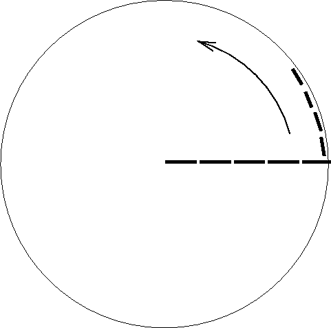 |
Fig. 3. Metre-sticks placed along the
circumference of the rotating disk are Lorentz-contracted, while those
placed along the radius are not effected.
Suppose we are in an inertial frame. Consider a big circular disk of radius
\(R\) which rotates with a uniform angular velocity \(\omega\) around its symmetry
axis perpendicular to its plane.
Suppose that \(R\omega < c\).
There are observers on the disk who measure the length of the perimeter and
radius of the disk by their metre-sticks.
The ratio of the perimeter to the radius would obviously be \(2\pi\) if both
quantities were measured in the inertial system,
since lengths were then measured between simultaneous
events (spacetime points). This was equivalent with
mapping the disk to a circle in the inertial frame,
and performing length measurements on that circle.
This ratio is different if the measurement is performed by the observers
staying on the disk. If they measure the perimeter,
their sticks are effected by Lorentz-contraction,
the contraction rate being \(\sqrt{1-R^2\omega^2/c^2}\) so
the observers find that the perimeter is \(2\pi
R/\sqrt{1-R^2\omega^2/c^2}\) (longer than \(2\pi R\),
while they find the radius to be the same \(R\) as
measured in the inertial frame. Hence on the disk,
in the co-rotating frame the ratio of perimeter to
radius is \(2\pi
/\sqrt{1-R^2\omega^2/c^2}>2\pi\). Thus, in an accelerating frame spatial
geometry is no longer Eucledian, and spacetime geometry is no longer Minkowskian.
Consider the interval between two nearby spacetime points. In the inertial
frame introduce Cartesian spatial coordinates \(dx'\), \(dy'\), \(dz'\), \(dt'\)
and cylindrical coordinates
\(dr'\), \(d\varphi'\), \(dz'\), \(dt'\). The interval is
\[\begin{align}
ds^2=c^2dt'^2-dx'^2-dy'^2-dz'^2=c^2dt'^2-dr'^2-r'^2d\varphi'^2-dz'^2\;.
\end{align}\]
Let us switch to the frame comoving with the disk by the transformation
\[\begin{align}
t' & = t \\
r' &= r \\
\varphi' &= \varphi +\omega t \\
z' &= z \phantom{forgkr1}
\end{align}\]
This ensures that constant unprimed spatial coordinates describe comoving
points, albeit the physical meaning (relation to measurements) is not obvious.
For the interval we get
\[\begin{align}
ds^2=\left(c^2-r^2\omega^2\right)dt^2-dr^2-r^2d\varphi^2-dz^2-2 r^2\omega d\varphi dt\;.
\end{align}\]
Invariance of the interval was assumed like in special relativity.
Clearly for an arbitrary coordinate transform the interval is a quadratic form
of coordinate differentials:
\[\begin{align}
ds^2=g_{ik}dx^idx^k\;.
\end{align}\]
The quantity \(g_{ik}\) is called the metric tensor. In the previous example
with coordinates \(x^0=ct\), \(x^1=r\), \(x^2=\varphi\) and \(x^3=z\) we have for
the nonzero components:
\[\begin{align}
g_{00} &= 1-r^2\omega^2/c^2 \\
g_{11} &= g_{33}=-1 \\
g_{22} &= -r^2 \\
g_{02} &= g_{20}=-r^2\omega/c\;.\phantom{forgmetrik1}
\end{align}\]
From the mathematical point of view the metric tensor is a \(4\times 4\) symmetric matrix. Signature (signs of the eigenvalues) plays a distinguished
role. A physically meaningful metric must have three negative and one positive
eigenvalues.
Curved coordinates
Why curved coordinates? Because
- in accelarating frames or in gravitational fields the metric is non-eucledian and
non-minkowskian,
- the main goal of the theory is to achieve a formulation equally valid in
arbitrary coordinate systems.
Suppose we are given an inertial frame. Starting with the expression of Minkowski interval
\[\begin{align}
ds^2=\left(dx'^0\right)^2-\left(dx'^1\right)^2-\left(dx'^2\right)^2-\left(dx'^3\right)^2
\end{align}\]
we transform it to curvilinear coordinates:
\[\begin{align}
x'^i=x'^i(x^0,x^1,x^2,x^3)\;.
\end{align}\]
Here primed coordinates are some (usually nonlinear) functions of the
unprimed ones. Thus we have
\[\begin{align}
dx'^i=\frac{\partial x'^i}{\partial x^j}dx^j\;,\phantom{kon_vek}
\end{align}\]
and
\[\begin{align}
ds^2=g_{ik}dx^idx^k\;,
\end{align}\]
where the metric tensor\(g_{ik}\)is given by
\[\begin{align}
g_{ik}=\frac{\partial x'^l}{\partial x^i}\frac{\partial x'^m}{\partial x^k}g_{lm}^{(0)}\phantom{f1}\;.
\end{align}\]
Here \(g_{lm}^{(0)}={\rm diag}\left(1,-1,-1,-1\right)\) stands for the Minkowski
metric. Since this transform is generally nonlinear, components \(g_{ik}\) depend on the coordinates. Vica versa, this means that in an accelerating
frame one may transform the metric simultaneously at all spacetime point to
Minkowski metric. This property is no longer true in gravitational fields
created by masses. In this case we say that spacetime is curved, since the
non-Minkowskian form is an inherent property of spacetime. Mathematically it
is obvious that if the ten independent components of the metric tensor are
arbitrary functions of spacetime, one cannot transform all of them to the
Minkowskian form, since a general coordinate transform involves only four
spacetime functions.
By inverting the previous expression we have
\[\begin{align}
g'_{lm}=\frac{\partial x^i}{\partial x'^l}\frac{\partial x^k}{\partial x'^m}g_{ik}\;.\phantom{f2}
\end{align}\]
Components of the metric tensor transform differently than coordinate
differentials (or products of coordinate differentials). Consider the
transformation rule of gradient of some scalar function \(\Phi(\{x^{i}\})\) We have
\[\begin{align}
\frac{\partial \Phi}{\partial x'^i}=\frac{\partial x^j}{\partial x'^i}\frac{\partial \Phi}{\partial x^j}\;,\phantom{kov_vek}
\end{align}\]
Quantities transforming according to the linear homogeneous transformation
rule of coordinate differentials will be called contravariant vectors
while those transforming like gradients of scalars will be called covariant vectors.
The transformation rule to apply will be denoted via index positions, namely,
a four component quantity with upper index stands for a contravariant vector,
while a lower index quantity is a covariant vector. Especially, each index of
the metric tensor transforms like a covariant vector. We call a
quantity with multiple indices a tensor whose components transform like
products of covariant and/or contravariant vector components.
The coefficient matrices of the two kinds of transformation rules are just the
inverses of each other. Therefore, contracting the indices of a covariant and
a contravariant vector yields a scalar:
\[\begin{align}
A'^iB'_i=\frac{\partial x'^i}{\partial x^k}A^k\frac{\partial x^n}{\partial x'^i}B_n=A^kB_k\;.\phantom{gk1}
\end{align}\]
In case of tensors, contracting a covariant index with a contravariant one
decreases the rank of the tensor by two.
By multiplying a contravariant vector \(A^k\) with the metric tensor
\(g_{ik}\) and summing over \(k\) we get a covariant vector denoted by \(A_i\) as it is
considered the covariant version of the same quantity \(A\)
\[\begin{align}
A_i=g_{ik}A^k\;.\phantom{gk2}
\end{align}\]
Vica versa, a covariant vector yields a contravariant one upon multiplication
(and index contraction) with the inverse of \(g_{ik}\). The inverse of the
metric tensor is denoted by \(g^{ik}\). It will be called contravariant metric tensor.
\[\begin{align}
A^i&=g^{ik}A_k\;,\phantom{gk3a}\\
g^{ik}g_{kj}&=\delta^i_j\;.\phantom{gk3b}
\end{align}\]
The procedure of creating a covariant quantity out of a contravariant one will
be called briefly lowering the index or pulling down the index, while the
opposite procedure will be called rising the index or pulling up the index.
Distances and elapsed times, proper physical quantities
Curved coordinates determine events in spacetime, but their diferences do not
correspond to proper distances or elapsed times. This is already the case when
using e.g. spherical coordinates. Questions:
- How to determine elapsed proper time between two nearby event, given the metric?
- How to determine proper distance between two nearby event, given the metric?
- How to determine a proper physical quantity corresponding to a vector or tensor, given the metric?
Basic principle: at the given spacetime point transform quantities to a local
inertial system, comoving with the given point. Proper quantities are given
in this tangent space.
Elapsed time between events which happened at the same spatial point
Suppose that \[dx^\alpha =0\quad (\alpha=1,2,3)\;.\]
The two events happen at the same spatial point in the comoving local inertial
system, too. Proper time \(d\tau\) elapsed between the events is related to the interval:
\[\begin{align}
ds^2=c^2d\tau^2\;.
\end{align}\]
Due to the invariance of the interval we have in curved coordinates
\[\begin{align}
ds^2=g_{00}\left(dx^0\right)^2\;,
\end{align}\]
which implies
\[\begin{align}
d\tau=\frac{\sqrt{g_{00}}}{c}dx^0\;.
\end{align}\]
Spatial distance between events
This time we have to construct the transformation to a local comoving inertial
frame. We apply a linear, homogeneous coordinate transformation which casts
the metric to Minkowski form. Further, we require that the inertial system is
comoving, which means that spatial coordinate differentials \(dx'^\alpha\) in
the inertial frame do not depend on \(dx^0\). Indeed, this condition ensures
that \(dx^\alpha=0\) implies \(dx'^\alpha=0\).
\[\begin{align}
dx'^\alpha&=A^\alpha_\beta dx^\beta\phantom{transz1}\\
dx'^0&= A^0_j dx^j\;.\phantom{transz2}
\end{align}\]
Greek letters stand for spatial indices (1,2,3) while Latin indices for
spatime indices (0,1,2,3).
Interval:
\[\begin{align}
ds^2=\left(dx'^0\right)^2-\left(dx'^\alpha\right)^2=A^0_j A^0_k
dx^jdx^k-A^\alpha_\beta A^\alpha_\nu dx^\beta dx^\nu\;.
\end{align}\]
This must coincide with
\(g_{jk}dx^jdx^k\) hence
\[\begin{align}
g_{00}&=\left(A^0_0\right)^2\phantom{g00}\\
g_{0\alpha}&=A^0_0A^0_\alpha\phantom{g01}\\
g_{\beta\nu}&=A^0_\beta A^0_\nu - A^\alpha_\beta A^\alpha_\nu\;.\phantom{g11}
\end{align}\]
The first equation implies
\[\begin{align}
A^0_0=\sqrt{g_{00}}\;,\phantom{a00}
\end{align}\]
while the second implies
\[\begin{align}
A^0_\alpha=\frac{g_{0\alpha}}{\sqrt{g_{00}}}\;.\phantom{a01}
\end{align}\]
When measuring distance \(d\ell\) we consider simultaneous events, i.e.,
we assume \(dx'^0=0\). Hence we have
\[\begin{align}
ds^2=-\left(d\ell\right)^2\phantom{tav1}
\end{align}\]
and
\[\begin{align}
dx'^0= A^0_j dx^j=0\;,
\end{align}\]
which is the condition of simultaneity in curved coordinates. Inserting the
elements of the transformation matrix we get
\[\begin{align}
dx^0=-\frac{g_{0\alpha}}{g_{00}}dx^\alpha\;.\phantom{szink1}
\end{align}\]
Synchronization of clocks. Simultaneity may be defined along curves in
spacetime, yet not along closed curves. Due to this latter, simultaneity of two events
separated by a finite distance cannot be defined. This happens in e.g. a
rotating frame:
\[\begin{align}
\Delta x^0=-\oint \frac{g_{0\alpha}}{g_{00}}dx^\alpha=\frac{2\pi R^2\omega c}{c^2-R^2\omega^2}
\end{align}\]
This property is a feature of the chosen frame and not of spacetime (the
latter is plane here). Actually, by a suitable coordinate transformation one
may set the three components \(g_{0\alpha}\) to zero and \(g_{00}\) to unity. The
resulting coordinate system is called synchronized. Then \(x^0\) is proper time everywhere
("world time").
As for proper distance, we have
\[\begin{align}
\left(d\ell\right)^2&=-ds^2=-g_{00}\left(dx^0\right)^2-2g_{0\alpha}dx^0dx^\alpha-g_{\alpha\beta}dx^\alpha
dx^\beta \\
&=\left(\frac{g_{0\alpha}g_{0\beta}}{g_{00}}-g_{\alpha\beta}\right)dx^\alpha
dx^\beta\;.
\end{align}\]
Spatial metric:
\[\begin{align}
\gamma_{\alpha\beta} =\frac{g_{0\alpha}g_{0\beta}}{g_{00}}-g_{\alpha\beta}\phantom{gamma}
\end{align}\]
This is just the inverse of \(-g^{\alpha\beta}\).
In case of rotating frame we get
for the nonzero components of spatial metric
\[\begin{align}
\gamma_{11}&=1 \\
\gamma_{22}&=\frac{r^2}{1-\frac{r^2\omega^2}{c^2}} \\
\gamma_{33}&=1\phantom{forgmetrik2}
\end{align}\]
According to this, the proper radius of the disk is \(R\) (independent of rotation),
while its proper circumference is \(2\pi
R/\sqrt{1-R^2\omega^2/c^2}\).
Proper physical quantities
Vectors and tensors may be given in curved coordinate systems in terms of their
contravariant or covariant components. The proper (actually measured) values
are those in the local comoving inertial frame. To this end have to transform
the curved components to this frame, and we shall need the quantities
\(A^\alpha_\beta\) as well. Given the conditions this is still ambiguous, since
the \(x\), \(y\), \(z\) spatial axes of the inertial frame may be arbitrarily
rotated. Indeed, we have
\[\begin{align}
A^\alpha_\beta A^\alpha_\nu=\gamma_{\beta\nu}\;,\phantom{transz2a}
\end{align}\]
whose solution is
\[\begin{align}
A^\alpha_\beta =F^\alpha_\nu\sqrt{\lambda_\nu} O^\nu_\beta \;,\phantom{transz3}
\end{align}\]
where \(F^\alpha_\nu\) stands for an arbitrary \(3\times 3\) orthogonal matrix
(rotation matrix), further, \(\lambda_\nu\) and \(O^\nu_\beta\) stand for the \(\nu\)-th eigenvalue and eigenvector
of the positive definite real symmetric matrix \(\gamma_{\alpha\beta}\), respectively.
As an example, let us calculate the proper velocity components of a point mass
on the rotating disk in terms of the time derivatives of its coordinates. Let
us denote the derivatives with respect to \(t\) by \(\dot{r}\),
\(\dot{\varphi}\) and \(\dot{z}\)
The components of the four velocity \(u^i=dx^i/ds\) are
\[\begin{align}
u^0&=\frac{dx^0}{ds}=\frac{1}{\sqrt{1-\frac{\dot{r}^2}{c^2}-\frac{r^2\left(\dot{\varphi}+\omega\right)^2}{c^2}-\frac{\dot{z}^2}{c^2}}}
\\
u^1&=\frac{dx^1}{ds}=\frac{\dot{r}}{c\sqrt{1-\frac{\dot{r}^2}{c^2}-\frac{r^2\left(\dot{\varphi}+\omega\right)^2}{c^2}-\frac{\dot{z}^2}{c^2}}} \\
u^2&=\frac{dx^2}{ds}=\frac{\dot{\varphi}}{c \sqrt{1-\frac{\dot{r}^2}{c^2}-\frac{r^2\left(\dot{\varphi}+\omega\right)^2}{c^2}-\frac{\dot{z}^2}{c^2}}}\\
u^3&=\frac{dx^3}{ds}=\frac{\dot{z}}{c\sqrt{1-\frac{\dot{r}^2}{c^2}-\frac{r^2\left(\dot{\varphi}+\omega\right)^2}{c^2}-\frac{\dot{z}^2}{c^2}}}
\end{align}\]
Since the spatial metric is already diagonal, \(O^\nu_\beta\) is the unit
matrix and the eigenvalues \(\lambda_\nu\) are just the diagonal elements of the
spatial metric. We
choose the arbitrary rotation matrix \(F^\alpha_\nu\) to be the unit matrix, too.
Then we get for the four vector components in the local comoving inertial frame
\[\begin{align}
u'^0&=\frac{dx'^0}{ds}=\frac{1-\frac{r^2\omega^2}{c^2}-\frac{r^2\omega\dot{\varphi}}{c^2}}{\sqrt{1-\frac{r^2\omega^2}{c^2}}\sqrt{1-\frac{\dot{r}^2}{c^2}-\frac{r^2\left(\dot{\varphi}+\omega\right)^2}{c^2}-\frac{\dot{z}^2}{c^2}}} \\
u'^1&=\frac{dx'^1}{ds}=\frac{\dot{r}}{c\sqrt{1-\frac{\dot{r}^2}{c^2}-\frac{r^2\left(\dot{\varphi}+\omega\right)^2}{c^2}-\frac{\dot{z}^2}{c^2}}} \\
u'^2&=\frac{dx'^2}{ds}=\frac{r\dot{\varphi}}{c\sqrt{1-\frac{r^2\omega^2}{c^2}}\sqrt{1-\frac{\dot{r}^2}{c^2}-\frac{r^2\left(\dot{\varphi}+\omega\right)^2}{c^2}-\frac{\dot{z}^2}{c^2}}} \\
u'^3&=\frac{dx'^3}{ds}=\frac{\dot{z}}{c\sqrt{1-\frac{\dot{r}^2}{c^2}-\frac{r^2\left(\dot{\varphi}+\omega\right)^2}{c^2}-\frac{\dot{z}^2}{c^2}}}
\end{align}\]
Here covered distances are measured in terms of proper time of the point
mass, as usual in case of four velocities. However, the components of proper
three velocities are measured in proper time of the disk, by clocks
synchronized along the trajectory of the particle. This means that
the proper elapsed time corresponding to \(dx^0\) is
\[\begin{align}
\frac{\sqrt{g_{00}}}{c}\left(dx^0+\frac{g_{0\alpha}}{g_{00}}dx^\alpha\right)\;,
\end{align}\]
since one has to consider that in the other spatial point time 0 is
simultaneous with \(-\frac{g_{0\alpha}}{g_{00}}dx^\alpha\).
This, however, means that one has to take the derivatives of the coordinates
with respect to \(dx'^0\). Thus the proper three velocity components:
\[\begin{align}
v^1&=c\frac{u'^1}{u'^0}=\frac{\dot{r}\sqrt{1-\frac{r^2\omega^2}{c^2}}}{1-\frac{r^2\omega^2}{c^2}-\frac{r^2\omega\dot{\varphi}}{c^2}} \\
v^2&=c\frac{u'^2}{u'^0}=\frac{r\dot{\varphi}}{1-\frac{r^2\omega^2}{c^2}-\frac{r^2\omega\dot{\varphi}}{c^2}}\\
v^3&=c\frac{u'^3}{u'^0}=\frac{\dot{z}\sqrt{1-\frac{r^2\omega^2}{c^2}}}{1-\frac{r^2\omega^2}{c^2}-\frac{r^2\omega\dot{\varphi}}{c^2}}
\end{align}\]
bene@arpad.elte.hu