Dr. Gyula Bene Department for Theoretical Physics, Loránd Eötvös University Pázmány Péter sétány 1/A, 1117 Budapest 4. week
Riemannian (curvature tensor)
Parallel displacement of a vector along a closed curve. Curvature
tensor. Symmetries of the Riemannian. Bianchi identity. Weil tensor, Ricci
tensor, scalar curvature. Example: calculating the Riemannian on a curved two
dimensional surface. Number of independent tensor components in two, three and
four dimensions.
Curvature tensor
Problem: what local quantity signals that spacetime is curved?
Parallel displacement of a vector: components in a locally Minkowskian
spacetime are unchanged. In curved spacetime:
\[\begin{align}DA^i=0\end{align}\]
During parallel displacement along a geodesics (\(Du^i=0\))
the angle made with the tangent of the trajectory (\(u^i\))is constant.
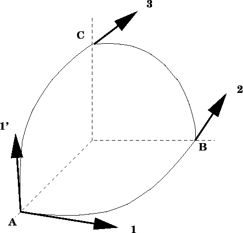
Parallel displacement along a closed curve:
Fig. 4.1. On a curved surface parallel
displacement along a closed curve does not reproduce the original vector.
\[\begin{align}
\Delta A_k=\oint \Gamma^i_{\phantom{1}kl}A_i dx^l
\end{align}\]
\[\begin{align}
\frac{\partial A_i}{\partial x^l}=\Gamma^n_{\phantom{1}il}A_n
\end{align}\]
Stokes's theorem:
\[\begin{align}
\oint A_i\;dx^i=\int df^{ki}\frac{\partial A^i}{\partial x^k}
=
\frac{1}{2}\int df^{ki}\left(\frac{\partial A^i}{\partial x^k}-\frac{\partial A^k}{\partial x^i}\right)
\end{align}\]
where
\[\begin{align}df^{ki}=dx^{(1) k}dx^{(2) i}-dx^{(1) i}dx^{(2) k}\end{align}\]
stands for the surface of the parallelogram spanned by the vectors \(dx^{(1) i}\) and \(dx^{(2) i}\).
\[\begin{align}
\Delta A_k=\frac{1}{2}\left[
\frac{\partial \left(\Gamma^i_{\phantom{1}km} A_i\right)}{\partial x^l}-
\frac{\partial \left(\Gamma^i_{\phantom{1}kl} A_i\right)}{\partial x^m}
\right]\Delta f^{lm}
\end{align}\]
\[\begin{align}
\Delta A_k=\frac{1}{2}{\mathcal R}^i_{\phantom{1}klm}A_i \Delta f^{lm}
\end{align}\]
\[\begin{align}
{\mathcal R}^i_{\phantom{1}klm}=
\frac{\partial \Gamma^i_{\phantom{1}km} }{\partial x^l}
-\frac{\partial \Gamma^i_{\phantom{1}kl} }{\partial x^m}
+\Gamma^i_{\phantom{1}nl}\Gamma^n_{\phantom{1}km}-\Gamma^i_{\phantom{1}nm}\Gamma^n_{\phantom{1}kl}
\end{align}\]
Expressing the Riemannian in terms of Christoffel symbols:
\[\begin{align}
{\mathcal R}^i_{\phantom{1}klm}A_i&=
\frac{\partial \left(\Gamma^i_{\phantom{1}km} A_i\right)}{\partial x^l}-
\frac{\partial \left(\Gamma^i_{\phantom{1}kl} A_i\right)}{\partial x^m} \\
&=\left(\frac{\partial \Gamma^i_{\phantom{1}km}}{\partial x^l}-
\frac{\partial \Gamma^i_{\phantom{1}kl} }{\partial x^m}\right) A_i
+\Gamma^i_{\phantom{1}km} \Gamma^n_{\phantom{1}il}A_n- \Gamma^i_{\phantom{1}kl}\Gamma^n_{\phantom{1}im}A_n \\
&=\left(\frac{\partial \Gamma^i_{\phantom{1}km}}{\partial x^l}-
\frac{\partial \Gamma^i_{\phantom{1}kl} }{\partial x^m}
+\Gamma^n_{\phantom{1}km} \Gamma^i_{\phantom{1}nl}- \Gamma^n_{\phantom{1}kl}\Gamma^i_{\phantom{1}nm}
\right) A_i
\end{align}\]
We made use that
\[\begin{align}
\frac{\partial A_i}{\partial x^l}=\Gamma^n_{\phantom{1}il}A_n
\end{align}\]
The derivation is valid for an arbitrary vector \(A_i\), hence
\[\begin{align}{\mathcal R}^i_{\phantom{1}klm}=\frac{\partial \Gamma^i_{\phantom{1}km}}{\partial x^l}-
\frac{\partial \Gamma^i_{\phantom{1}kl} }{\partial x^m}
+\Gamma^n_{\phantom{1}km} \Gamma^i_{\phantom{1}nl}- \Gamma^n_{\phantom{1}kl}\Gamma^i_{\phantom{1}nm}\end{align}\]
Properties of the Riemannian
Change of a contravariant vector along an infinitesimally small closed surface
\[\begin{align}
{\mathcal R}=\frac{2{\mathcal R}_{1212}}{\gamma}
\end{align}\]
\[\begin{align}
\frac{{\mathcal R}}{2}=K=\frac{1}{\rho_1\rho_2}
\end{align}\]
where \(\rho_1\) and \(\rho_2\) stand for the principal curvature radii. Proof:
Choose a Cartesian coordinate system at a point \(P\) of a two dimensional surface,
embedded into a three dimensional Eucledian frame so that
Point \(P\) is the origin
Axis \(z\) is normal to the surface
Planes \(xz\) and \(yz\) are the planes of principal curvatures.
The equation of the surface in a small neighborhood of the origin:
\[\begin{align}
z=\frac{x^2}{2\rho_1}+\frac{y^2}{2\rho_2}\;.
\end{align}\]
Surface metric is derived from the distance of two nearby surface points:
\[\begin{align}
ds^2&=dx^2+dy^2+dz^2=dx^2+dy^2+\left(\frac{xdx}{\rho_1}+\frac{ydy}{\rho_2}\right)^2 \\
&=\left(1+\frac{x^2}{\rho_1^2}\right)dx^2+\left(1+\frac{y^2}{\rho_2^2}\right)dy^2+2\frac{xy}{\rho_1\rho_2}dxdy\;,
\end{align}\]
thus
\[\begin{align}
g_{11}&=1+\frac{x^2}{\rho_1^2}\;,\\
g_{12}&=g_{21}=\frac{xy}{\rho_1\rho_2}\;,\\
g_{22}&=1+\frac{y^2}{\rho_2^2}
\;.
\end{align}\]
First derivatives vanish at the origin, and the metric is the unit matrix
there. Then we have
\[\begin{align}
{\mathcal R}_{1212}(0)=\frac{\partial^2 g_{12}}{\partial x \partial y}-\frac{1}{2}\frac{\partial^2 g_{11}}{\partial y^2}-\frac{1}{2}\frac{\partial^2 g_{22}}{\partial x^2}=\frac{1}{\rho_1\rho_2}\;.
\end{align}\]
Q.E.D.
Bianchi's identity
\[\begin{align}
{\mathcal R}^n_{\phantom{1}ikl;m}+{\mathcal R}^n_{\phantom{1}imk;l}+{\mathcal R}^n_{\phantom{1}ilm;k}=0\phantom{bian1}
\end{align}\]
Proof:
\[\begin{align}
{\mathcal R}^n_{\phantom{1}ikl;m}+{\mathcal R}^n_{\phantom{1}imk;l}+{\mathcal R}^n_{\phantom{1}ilm;k}=\frac{1}{2}{\mathcal R}^n_{\phantom{1}ikl;m}E^{klmp}\sqrt{-g}\end{align}\]
where \[\begin{align}E^{klmp}=\frac{1}{\sqrt{-g}}e^{klmp}\end{align}\]
The cyclic sum multiplied by \(1/\sqrt{-g}\) is a tensor. Switching to a locally
geodetic (Minkowskian) frame we have
\[\begin{align}
{\mathcal R}^n_{\phantom{1}ikl;m}=\frac{\partial {\mathcal R}^n_{\phantom{1}ikl}}{\partial x^m}
=\frac{\partial^2 \Gamma^n_{\phantom{1}il}}{\partial x^m \partial x^k}
-\frac{\partial^2 \Gamma^n_{\phantom{1}ik}}{\partial x^m \partial x^l}\end{align}\]
This implies
\[\begin{align}
{\mathcal R}^n_{\phantom{1}ikl;m}+{\mathcal R}^n_{\phantom{1}imk;l}+{\mathcal R}^n_{\phantom{1}ilm;k}
&=\frac{\partial^2 \Gamma^n_{\phantom{1}il}}{\partial x^m \partial x^k}
-\frac{\partial^2 \Gamma^n_{\phantom{1}ik}}{\partial x^m \partial x^l} \\
&+\frac{\partial^2 \Gamma^n_{\phantom{1}ik}}{\partial x^l \partial x^m}
-\frac{\partial^2 \Gamma^n_{\phantom{1}im}}{\partial x^l \partial x^k} \\
&+\frac{\partial^2 \Gamma^n_{\phantom{1}im}}{\partial x^k \partial x^l}
-\frac{\partial^2 \Gamma^n_{\phantom{1}il}}{\partial x^k \partial
x^m}=0\end{align}\]
Q.E.D.
Bianchi's identity implies by contracting indices \(i\) with \(k\) and \(n\) with \(l\):
\[\begin{align}
0=g^{ik}\left({\mathcal R}^l_{\phantom{1}ikl;m}+{\mathcal R}^l_{\phantom{1}imk;l}+{\mathcal R}^l_{\phantom{1}ilm;k}\right)=-{\mathcal R}_{,m}+2{\mathcal R}^l_{\phantom{1}m;l}
\end{align}\]
or
\[\begin{align}{\mathcal R}^l_{\phantom{1}m;l}=\frac{1}{2}\frac{\partial {\mathcal R}}{\partial x^m}\phantom{bian2}\end{align}\]
Number of components of the Riemannian
Two dimensional case:
a single independent component, eg. \({\mathcal R}_{1212}\).
Three dimensional case:
\({\mathcal R}_{\alpha\beta\gamma\delta}\)'s
first (\(\alpha\beta\)) and second
(\(\gamma\delta\)) pairs of indices take on three values each, hence the number
of independent components is the same as that of a symmetric \(3\times 3\)
matrix, that is 6. (Cyclic sum vanishes automatically, without implying any further restrictions.)
Four dimensional case:
\({\mathcal R}_{iklm}\)'s first (\(ik\)) and second
(\(lm\)) pairs of indices take on six values each. The number of independent
components of a \(6\times 6\) symmetric matrix is 21. Cyclic sum vanishes
automatically, except when all the four indices are different. In that latter
case we have a single further algebraic restriction among components, reducing
the number of independent components to 20.
Weil's tensor:
\[\begin{align}C_{iklm}={\mathcal R}_{iklm}-\frac{1}{2}{\mathcal R}_{il}g_{km}+\frac{1}{2}{\mathcal R}_{im}g_{kl}+\frac{1}{2}{\mathcal R}_{kl}g_{im}-\frac{1}{2}{\mathcal R}_{km}g_{il}+\frac{1}{6}{\mathcal R}\left(g_{il}g_{km}-g_{im}g_{kl}\right)\end{align}\]
It possesses all the algebraic symmetries of the Riemannian, but contracting
any two indices we get zero (irreducible tensor).
bene@arpad.elte.hu